What is a System Resistance Curve for a Pump?
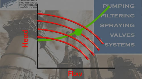
The pump system resistance curve is a graphical representation of the relationship between the pump's flow rate and the total head (pressure) the pumping system requires.
This curve shows the relationship between the flow rate and the total dynamic head (TDH) that the pump must overcome to deliver the fluid through the system. To create a pump system resistance curve, engineers and technicians need to calculate the system curve, which represents the hydraulic characteristics of the system, and the pump curve, which represents the pump's performance.
The pump system resistance curve is crucial for designing, installing, and operating pump systems that are efficient, reliable, and cost-effective.
Understanding a System Resistance curve can help us:
- Select a pump that will deliver the required flow rate at the appropriate pressure.
- Help troubleshoot problems in existing systems.
- Identify areas of high-pressure drop and determine the cause of the problem, such as clogged pipes or undersized fittings.
- Optimize the performance of existing systems.
- Minimize pressure losses and improve overall system efficiency by analyzing the curve and adjusting the system's parameters, such as pipe diameter or valve settings.
What is the difference between a System Curve and a Pump Curve?
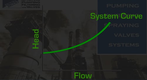
The system curve is a graph that shows the pressure or head required by the fluid system at different flow rates. It is determined by calculating the resistance to flow of all the components in the system, such as friction losses due to pipe diameter, length, and roughness; elevation changes; and fittings and valves. The system curve is fixed and does not change unless there is a change in the system's configuration or operating conditions.
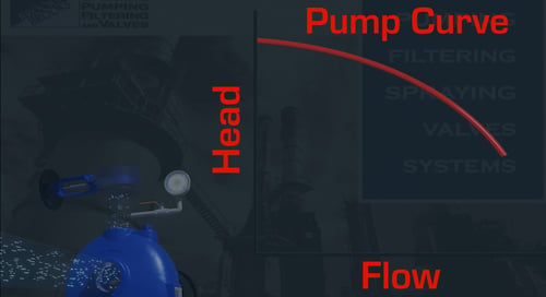
The pump curve is a graph that shows the pump's flow rate, head, and power consumption at different operating points. It is determined by conducting performance tests on the pump under controlled conditions. The pump curve is specific to the pump model and size and does not change unless there is a change in the pump's configuration or performance.
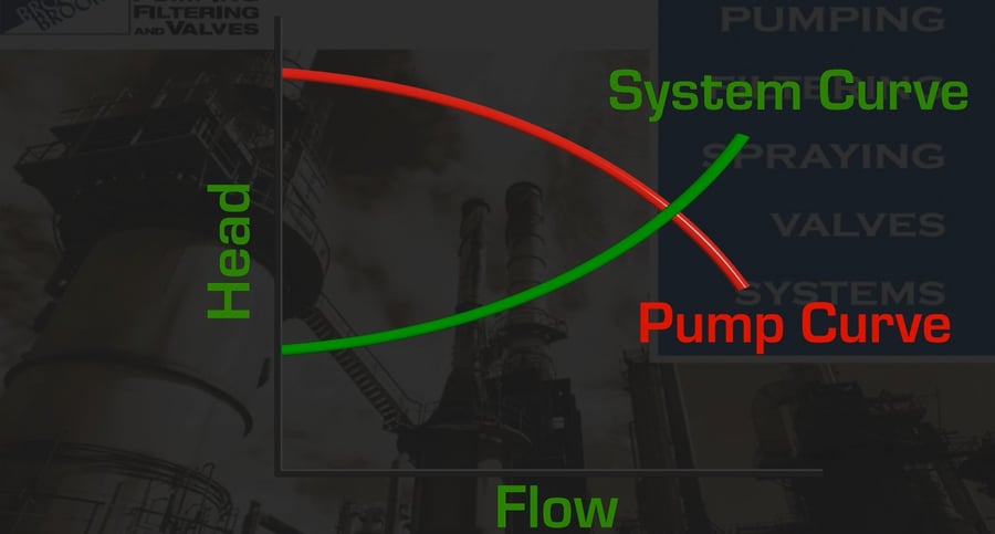
The pump curve and system curve are combined to create the pump system curve or total head curve, which shows the total head that the pump must overcome to deliver a specific flow rate through the system.
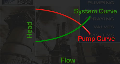
The intersection of the pump curve and the system curve represents the pump’s operating point, where the flow rate and head produced by the pump match the pressure or head required by the system. This assumes the pump is in a “like-new” condition, has no air entrainment, and is not suction cavitating.
To predict the pump’s operating points, we must first learn about the piping system the pump is connected to.
Pump System Resistance Curve Calculation
Calculating the total pressure drop in a piping system at carrying flow rates will give us a system resistance curve. Where this curve intersects the pump curve is where the pump should operate.
To calculate the system curve, we need to know two values:
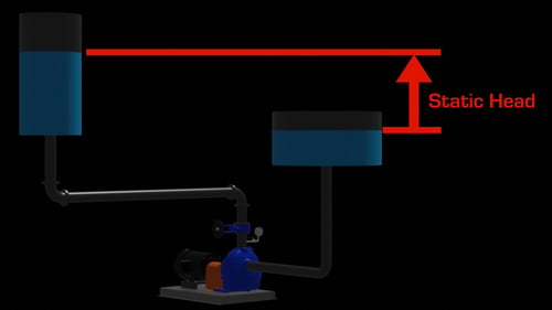
- The Static Head
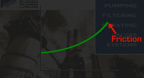
- The Frictional Losses
The static head is easy to measure. You only require a tape measure or an accurate system drawing. The vertical distance from the source of the liquid to its highest point in the system is the static head. Be careful of piping systems that angulate as syphons may develop.
Calculating the frictional losses involves a complete understanding of all the components in the system. For instance, the pipe length, diameter, material type, the type and number of valves and fittings, and any other equipment like filters, heat exchangers, or nozzles need to be accounted for.
All these components have their own system resistance curves that can be found in reference data. Usually, the manufacturer or supplier is the best place for this information.
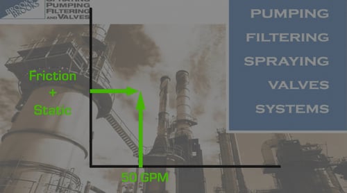
For example, we can reference commonly available tables to determine the frictional loss of a steel pipe. If we have a pipe that is 100 ft. long and 2 inches in diameter, with 50 GPM flowing through it, the frictional loss is estimated to be around 2 psi. As we increase this flow rate, the losses will also increase.
Similar relationships can also be found for the other components in the piping system.
How to Plot a System Resistance Curve for a Pump
Looking at the system, we can add the resistances together to get the total frictional losses. For instance, at a typical flow rate of 50 GPM, sum each of the components’ frictional losses together, add the static head, and plot this on the pump curve.
Repeat the process for other flow rates. We will have a system resistance curve if we connect all these points with a smooth line. Now we can estimate what pump speed or impeller diameter we should use to achieve a particular flow and head.
Now that we know the basics, we can analyze more complicated systems.
John Brooks Company is Your Prime Source for Pumps
John Brooks Company partners with world-renowned manufacturers to offer a variety of pumps for a broad range of commercial, municipal, and industrial uses, such as agriculture, food production, oil and gas, and mining. Our experts are available to assist you in selecting the right pump for your specific requirements.
Contact us now to explore what we have to offer or speak to one of our specialists.
.jpeg?width=500&name=AdobeStock_301608794%20(1).jpeg)